


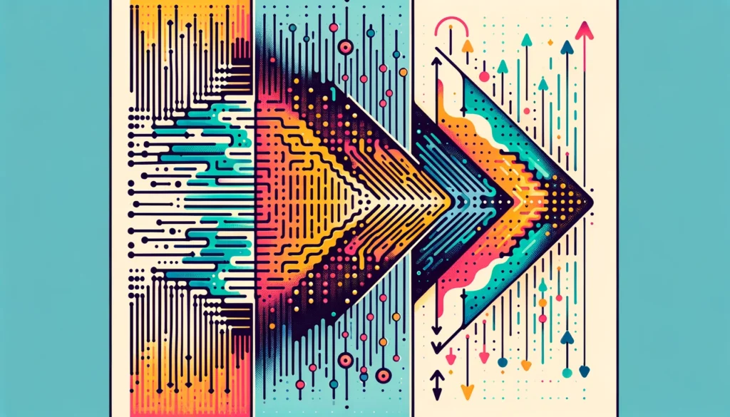
Mastering Gradient Descent: Optimizing Machine Learning
Gradient Descent is a method I’ve used a lot in my work with machine learning and artificial intelligence. It’s

Gradient Descent is a method I’ve used a lot in my work with machine learning and artificial intelligence.
It’s interesting how this algorithm, which is commonly used to train models, makes complicated issues easier to handle.
At its heart, gradient descent aims for optimization, changing parameters little by little to lower the mistakes between what is predicted and the actual outcomes.
With every iteration, it’s like watching a student learn, as each step brings the model nearer to its goal.
The cost function works like a barometer, checking how right the predictions are, always trying to get to the point where the mistake is almost zero.
It’s a way of minimizing the tiniest differences and improving the parameters to make the models work better.
This continuous search for optimization not only aids in training neural networks but also in creating strong tools for computer science and AI applications.
The joy of watching your model adjust and get better over time is huge, showing the real spirit of machine learning.
Types of Gradient Descent
In the world of gradient descent, an important idea in learning algorithms, there are three main types: batch gradient descent, stochastic gradient descent (SGD), and mini-batch gradient descent.
Each type has its way of making mistakes smaller and improving the model.
My experience with machine learning has taught me about these methods and how they each have a special role in making learning better.
Batch gradient descent goes the usual way, adding up the mistakes from all the examples we train with before changing the model once.
This way of doing things is steady and reaches the goal, but it can be slow, especially with a lot of data.
Then there is the stochastic way, where every training example is looked at and changed on its own, making learning fast and detailed but sometimes a bit messy.
Mini-batch gradient descent mixes a bit of both, making the computer work smarter and faster by changing in small batches.
This method finds a good mix between being quick and being thorough, aiming to get to the best solution, whether it’s a local or global minimum.
Also read: Starlink Internet: How It is Revolutionizing Internet Access
How Does Gradient Descent Work?
To get why gradient descent is useful, it helps to look back at linear regression, especially the part about the slope of a line equation, y = mx + b. Here, m is the slope and b is the intercept on the y-axis.
It is important because gradient descent is similar to finding the best straight line in statistics that fits our data, focusing on the error in guessing compared to the real values.
The main goal of gradient descent is to make this error smaller by changing the model’s parameters during iterations, making it work better.
The process starts at a random spot in our data graph, setting things up for gradient descent to check how steep the slope is using a tangent line.
This helps decide how to change the model’s weights and bias. The aim is to get to the bottom point on the cost function graph, called the convergence point, where the error between the real y and the guessed y is the smallest.
The learning rate is key here, controlling how big the steps are toward this lowest point to find the right mix of accuracy and speed.
With this step-by-step method, the model gets better, tweaking its parameters until the cost function is almost zero, showing the best learning.
Challenges of Gradient Descent
Gradient descent is an important way to make things better in machine learning, but it can be tricky.
One problem is with local minima and saddle points, especially in nonconvex problems. While convex problems let gradient descent easily find the global minimum (where the model does its best), nonconvex problems might make the algorithm get stuck in local minima or saddle points.
These points are like the part of a saddle you sit on, where the slope goes up one way but not the other, which makes it hard for the model to get out and find the real lowest point.
Another issue happens in big neural networks, like recurrent neural networks, where you might see vanishing gradients or exploding gradients.
With vanishing gradients, the model starts to learn slowly because the gradient gets too small, making the front parts of the network learn slower than the back parts.
This might make the model stop learning because the changes become too tiny.
On the other hand, exploding gradients can make the model’s weights get big, making things unstable and causing weird errors.
One way to deal with this is to use a dimensionality reduction method to make the model simpler and help keep the learning steady.
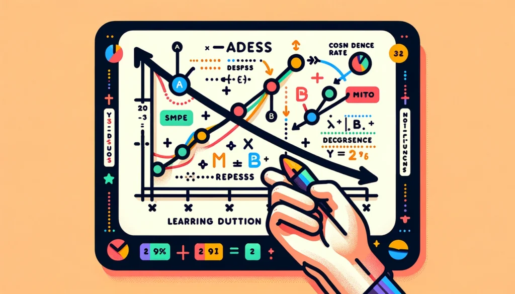
Plotting the Gradient Descent Algorithm
When we look at the gradient descent method, using pictures to show it can be very helpful.
For a parameter like theta, we usually draw the cost on the y-axis and theta on the x-axis.
If we have two parameters, we use a 3-D plot, which shows the cost on one axis and the two parameters on the other axes.
Another way to see this is with Contours, which shows a 3-D plot in two dimensions, where the change is shown as a contour.
Here, the value of the change gets bigger as you move away from the middle, stays the same in circles, and is linked to how far you are from the middle.
The Learning Rate (Alpha) is very important in this, as it decides how big and which way the steps we take toward the lowest point will be.
If the Learning Rate is too big, we might go past the lowest point, causing the method to jump around and not get there.
If the Learning Rate is too low, it makes the training take a very long time and not so good. A just-right Learning Rate helps the model get to the lowest point well.
If the Learning Rate is more than the best amount, it might get there but with the chance of going too far.
And if it’s really big, the method goes the wrong way and gets worse, not better.